Overview of Presentation
- Bayesian vs. frequentist inference
- Bayes’ Theorem
- Example of Bayesian inference
- Bayesian LMERs with rstanarm
- how to code models
- selecting priors
- displaying & interpreting the posterior distribution
- model diagnostics and comparisons
Bayesian vs. Frequentist Inference
Frequentist Inference
- Uses only the data and compares it to an idealized model to make inferences about the data
- Example Problem: You lose your cellphone in your house. You have a friend call it and you listen for the sound to find it. Where do you search in the house?
- Frequentist solution: You can hear the phone ringing. You also have a mental model of the house that helps you identify where the sound is coming from. When you hear the phone ringing, you infer the location with the help of your model.
Bayesian Inference
- Draws conclusions from data and all prior knowledge about the data including idealized models
- Uses prior knowledge to make bets on the outcome
- Bayesian solution: You can hear the phone ringing but you also know where you were today in the house and where you tend to lose things. You also have a mental model of the house. You combine the inferences from the ringing with your prior knowledge to find the phone
Bayes’ Theorem
- \(P(A\mid B) = \frac{P(B \mid A) \, P(A)}{P(B)}\)
- The probability of observing event A given that B is true equals the probability of observing event B given the A is true times the probability of observing event A divided by the probability of event B
- Can be reformulated as Bayes’ Rule:
- Prior Odds * Relative Likelihoods = Posterior Odds
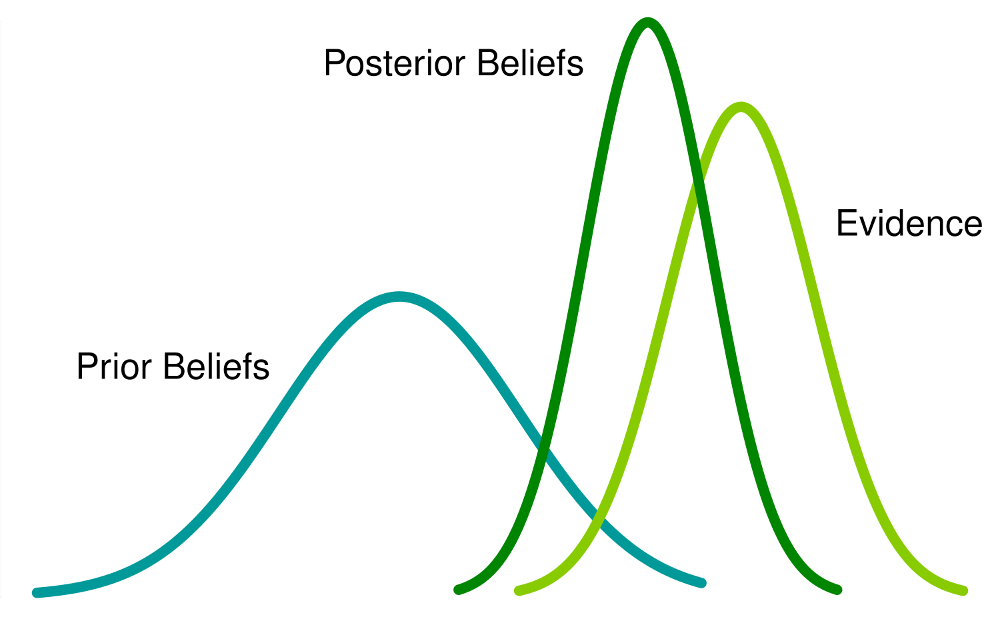
Bayesian Terms
- Prior odds = our beliefs about the events prior to looking at the new data
- Relative likelihoods = how likely an observation is when comparing one hypothesis to another
- Posterior odds = our state of belief after comparing the prior information to the likelihoods (and updating with new data)
What they look like
Applying Bayes’ Theorem: Example Problem
- You are treating students with Diseasitis
- 20% of students will have Diseasitis right now based on previous research
- You have a test that turns black if a student has Diseasitis
- If a student has Diseasitis, only 90% cause the test to turn black
- The test also turns black 30% of the time for healthy students
- A student comes in to take the test and it turns black. What is the probability they have Diseasitis?
Solution
- We know
- The probability of black given sick = 0.9
- The probability of black given not sick = 0.3
- The probability of sick = 0.2
- Prior odds X Relative likelihoods = Posterior odds
- Relative likelihoods compare the probabilities of the two observed outcomes (prob of black = sick and prob of black = healthy)
- \(\frac{P(sick)}{P(healthy)} \times \frac{P(black\mid sick)}{P(black\mid healthy)} = \frac{P(sick\mid black)}{P(healthy\mid black)}\)
- \((20\% : 80\%) \times (90\%:30\%) = \frac{3}{4}\) odds or \(\frac{3}{7} =43\%\) probability of sick given blackened test
- Remember: odds \((A:B)\) = probability \(\frac{A}{A+B}\)
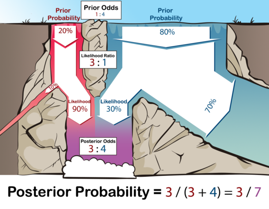
Solution (con’t)
- Another way to look at it:
- Imagine a waterfall with two different colored waters
- At the top of the waterfall, 20 gallons/second of red water are flowing down, and
- 80 gallons/second of blue water are coming down.
- 90% of the red water makes it to the bottom.
- 30% of the blue water makes it to the bottom.
- Of the purplish water that makes it to the bottom of the pool, how much was originally from the red stream and how much was originally from the blue stream?
Solution visualized
Applying Bayesian inference to LMERs
Applying Bayesian Inference
- Bayesian inference can be applied to most models (ANOVA, linear regression, GLMERs, LMERs, GAMMs, CLMMs, etc.)
- Bayesian inference does not give p-values (more on this later)
- It can run models that otherwise don’t converge with frequentist models
- Easier to intrepret
- Provide distribution of values for each parameter rather than a single output
Applying Bayesian Inference
- Real life language data is much more complex than the earlier examples
- We can’t directly calculate the posterior distribution
- Instead we have to approximate accurate posterior distributions
- The rstanarm package uses the Stan language to generate a posterior distribution via Markov chain Monte Carlo sampling
- This process takes time (sometimes a long time!) and requires thousands of samples
- Stan is much more efficient than BUGS or JAGS (other Bayesian samplers) and is in active development
rstanarm
- Use
library(rstanarm) stan_lmer()orstan_glmer()- Similar syntax to
lme4but have to specify - priors
- number of chains
- iterations
- adapt_delta (optional)
Selecting priors
- No matter what we research, we already know something about the data we will collect before we do
- For phonetics, we know range of sounds human can produce and hear
- We know that it is very unlikely to get meaningful speech sounds that are 100,000 Hz
- VOTs are typical not seconds long or conversely not extremely short like 1 ns
- We pick priors that are weakly informative but still helpful
- We want to make some bets but not bet too strongly to overly influence the results
- We pick priors that are distributions (typically normal) that have a reasonable mean and standard deviation but not too narrow nor too wide
Selecting priors
- The priors tell the model where to start guessing at the data and how strong of a bet to make
- If we have lots of data that strongly diverge from the priors, then the results won’t reflect the priors as much, but if the priors are too strong then they can heavily influence our results
VOT example
- We need to pick priors for the intercept and slopes for VOT data
- What do we know about VOT that are measured in ms?
- We can pick a prior with a normal distribution centered at 0ms with a standard deviation of 50ms: normal(0,50)
- that says we are 68% sure the mean is between -50ms and 50ms, 95% sure between -100ms and 100ms and 99.7% sure between -150ms and 150ms
- We can tweak it as needed
- What if we said normal(0,5)? Is that too strong? Or normal(0,500)? Is that too weak?
Sampling the posterior distribution
- We need to specify how many samples we need in addition to the number of chains
- Stan is quite efficient so we can use a relatively small amount depending on how nice the data are
- Typically use chains = 4 (number of unique samplers) and iter = 2000
- The sampling process requires warmup samples to get a taste of the distribution, which we throw out since not very good (warmup = 1000)
- Sometimes there are divergent samples which are bad so we add adapt_delta=0.999 (if still divergent keep adding 9s until it works)
Let’s make some models!
- These can take a bit of time to run
data_vot <- read_csv("t_d_vot.csv") # import data
options(mc.cores=parallel::detectCores ()) # Run on multiple cores
# strong priors
model1 <-stan_lmer(vot*1000 ~ consonant2 + (1+consonant2|speaker_id) + (1+consonant2|word),
                   data=data_vot,
                   prior_intercept = normal(0, 5,autoscale = F),
                   prior = normal(0, 5,autoscale = F),
                   prior_covariance = decov(regularization = 2),
                   chains = 4,
                   iter = 2000, adapt_delta=0.999,warmup=1000)
More models
# weaker priors
model2 <-stan_lmer(vot*1000 ~ consonant2 + (1+consonant2|speaker_id) + (1+consonant2|word),
                   data=data_vot,
                   prior_intercept = normal(0, 50,autoscale = F),
                   prior = normal(0, 50,autoscale = F),
                   prior_covariance = decov(regularization = 2),
                   chains = 4,
                   iter = 2000, adapt_delta=0.999,warmup=1000)
One last model
# very weak priors
model3 <-stan_lmer(vot*1000 ~ consonant2 + (1+consonant2|speaker_id) + (1+consonant2|word),
                   data=data_vot,
                   prior_intercept = normal(0, 500,autoscale = F),
                   prior = normal(0, 500,autoscale = F),
                   prior_covariance = decov(regularization = 2),
                   chains = 4,
                   iter = 2000, adapt_delta=0.999,warmup=1000)
Interpreting Results
What are p-values?
- From http://www.labstats.net/articles/pvalue.html
- The probability of getting the results you did (or more extreme results) given that the null hypothesis is true.
- P = 0.05 does not mean there is only a 5% chance that the null hypothesis is true.
- P = 0.05 does not mean there is a 5% chance of a Type I error (i.e. false positive).
- P = 0.05 does not mean there is a 95% chance that the results would replicate if the study were repeated.
- P > 0.05 does not mean there is no difference between groups.
- P < 0.05 does not mean you have proved your experimental hypothesis.
Intrepreting p-values
- If you are studying the difference in VOT between two stops and the p-value is 0.03 that means:
- if there were no difference between the VOT of the two stops, you’d get the observed difference or more in 3% of the studies due to random sampling error.
- It does not give us any information about the alternate hypothesis that there is a difference between the stops’ VOTs.
Bayesian Approach
- No p-values!
- Use Bayesian Highest Density Interval (HDI)
- Area of posterior distribution with 95% highest probability [2.5% to 97.5% of posterior distribution]
- Bayesian approach answers “The probability of the Null Hypothesis being true given the data” (Frequentist is “The probability of observing the data or anything more extreme given the null hypothesis”)
- Bayesian approach is more inuitive
- Multiple comparisons also aren’t an issue!
## Intrepreting HDI
- If there is no overlap of HDIs, then probable difference
- If overlap can say there is probable similarity but also probable difference (can now make these claims rather than just binary answers!)
- Much more nuanced and like real life
Model 1 Results
| mean | mcse | sd | 2.5% | 25% | 50% | 75% | 97.5% | n_eff | Rhat | |
|---|---|---|---|---|---|---|---|---|---|---|
| (Intercept) | 4.0864961 | 0.1266263 | 5.3324124 | -6.4999536 | 0.3921561 | 4.2270555 | 7.876507 | 14.26621 | 1773 | 1.0002057 |
| consonant2t̻ | 1.8167415 | 0.1058488 | 4.9799389 | -8.2129145 | -1.4335593 | 1.8672895 | 5.128587 | 11.62017 | 2213 | 1.0018490 |
| b[(Intercept) speaker_id:F01] | 6.1571967 | 0.3203016 | 6.6888620 | -5.5604391 | 1.1397537 | 5.8466621 | 10.632572 | 19.77066 | 436 | 1.0066978 |
| b[consonant2t̻ speaker_id:F01] | 9.2544098 | 0.8048084 | 13.0114306 | -12.3259024 | -1.6638371 | 8.2141599 | 20.560041 | 32.78133 | 261 | 1.0114576 |
| b[(Intercept) speaker_id:F02] | -0.1790354 | 0.3008634 | 6.5528716 | -11.9120906 | -4.7962143 | -0.5556100 | 4.051550 | 13.67538 | 474 | 1.0046269 |
| b[consonant2t̻ speaker_id:F02] | 21.2263520 | 0.8436341 | 13.4194616 | -0.6464893 | 9.8916638 | 19.9318661 | 32.997877 | 44.63413 | 253 | 1.0122115 |
| b[(Intercept) speaker_id:M01] | 20.8152190 | 0.3496184 | 7.1102001 | 8.1548843 | 15.6766691 | 20.6613122 | 25.518407 | 35.08725 | 414 | 1.0086930 |
| b[consonant2t̻ speaker_id:M01] | 3.1611167 | 0.7882159 | 12.9473913 | -19.1680871 | -7.3671564 | 1.7137774 | 14.332284 | 25.81529 | 270 | 1.0095255 |
| b[(Intercept) speaker_id:M02] | 3.8957675 | 0.3192612 | 6.7343050 | -7.9658212 | -0.9439335 | 3.3301208 | 8.467740 | 17.98618 | 445 | 1.0066537 |
| b[consonant2t̻ speaker_id:M02] | 6.6532391 | 0.8065003 | 12.9791396 | -14.9735835 | -4.1659549 | 4.9942416 | 17.983205 | 29.81430 | 259 | 1.0111424 |
| b[(Intercept) speaker_id:M03] | 8.3188733 | 0.3107234 | 6.7029312 | -3.5148628 | 3.5766378 | 7.8081863 | 12.810630 | 22.36286 | 465 | 1.0058295 |
| b[consonant2t̻ speaker_id:M03] | 30.0009369 | 0.8610039 | 13.8191725 | 7.5520796 | 18.1920717 | 28.9177002 | 42.115818 | 54.17208 | 258 | 1.0126060 |
| b[(Intercept) word:ahdan] | 1.4513173 | 0.1948404 | 5.2998150 | -7.2890099 | -1.2174846 | 0.1475008 | 3.250404 | 14.80495 | 740 | 1.0052302 |
| b[consonant2t̻ word:ahdan] | 0.4205744 | 0.2205275 | 13.9473834 | -30.6421033 | -3.4534170 | 0.0435104 | 4.419632 | 31.09333 | 4000 | 0.9995036 |
| b[(Intercept) word:ata] | 5.9983941 | 0.4610827 | 11.1459093 | -7.4882486 | -0.3187069 | 1.6672417 | 10.255426 | 35.63936 | 584 | 1.0064080 |
| b[consonant2t̻ word:ata] | 10.5945488 | 0.6598986 | 13.4471019 | -4.8164844 | 0.0128475 | 5.6905976 | 19.930322 | 41.17283 | 415 | 1.0053769 |
| b[(Intercept) word:idi] | 3.1229898 | 0.2239212 | 5.5562291 | -5.1150601 | -0.1005295 | 1.3810099 | 5.539898 | 17.20763 | 616 | 1.0051051 |
| b[consonant2t̻ word:idi] | 0.9119649 | 0.2231316 | 13.9709089 | -29.2847326 | -3.0776975 | 0.0763752 | 4.750007 | 32.42595 | 3920 | 1.0000484 |
| b[(Intercept) word:itik] | 7.0288940 | 0.4652301 | 11.2837918 | -6.8164340 | 0.0649321 | 2.6536150 | 11.458345 | 36.75228 | 588 | 1.0043226 |
| b[consonant2t̻ word:itik] | 12.4591581 | 0.7015108 | 13.8732923 | -3.1514511 | 0.6738726 | 7.9105136 | 22.269547 | 43.61696 | 391 | 1.0066493 |
| sigma | 6.3583149 | 0.0131140 | 0.6890298 | 5.1838229 | 5.8768264 | 6.2991658 | 6.749955 | 7.93253 | 2761 | 0.9994410 |
| Sigma[speaker_id:(Intercept),(Intercept)] | 196.8932077 | 6.2667480 | 181.8820568 | 27.6287381 | 77.7356439 | 139.5448053 | 251.700022 | 715.22591 | 842 | 1.0038181 |
| Sigma[speaker_id:consonant2t̻,(Intercept)] | 48.7473253 | 5.8044110 | 136.4071223 | -148.4347459 | -25.7137070 | 15.9920358 | 98.179490 | 403.26124 | 552 | 1.0049717 |
| Sigma[speaker_id:consonant2t̻,consonant2t̻] | 422.3109484 | 20.5367610 | 424.3029914 | 48.7769109 | 133.6042056 | 281.1530738 | 567.852549 | 1577.86463 | 427 | 1.0067827 |
| Sigma[word:(Intercept),(Intercept)] | 114.0889282 | 8.9331102 | 216.6859959 | 0.0340652 | 3.2356146 | 25.8367294 | 130.758542 | 747.66508 | 588 | 1.0048817 |
| Sigma[word:consonant2t̻,(Intercept)] | 16.6823899 | 2.0121354 | 95.1906538 | -146.4042270 | -1.7539351 | 0.6144948 | 29.869396 | 229.08762 | 2238 | 1.0003819 |
| Sigma[word:consonant2t̻,consonant2t̻] | 221.8939850 | 14.5030489 | 360.6208258 | 0.0355739 | 5.2610660 | 79.1953082 | 297.683633 | 1220.99980 | 618 | 1.0069617 |
| mean_PPD | 30.6615249 | 0.0183833 | 1.1626600 | 28.4549208 | 29.8770106 | 30.6501532 | 31.441122 | 32.93101 | 4000 | 0.9998124 |
| log-posterior | -239.0927218 | 0.1498344 | 4.9706903 | -249.6491694 | -242.1890713 | -238.6483981 | -235.576336 | -230.67157 | 1101 | 1.0002455 |
Model 2 Results
| mean | mcse | sd | 2.5% | 25% | 50% | 75% | 97.5% | n_eff | Rhat | |
|---|---|---|---|---|---|---|---|---|---|---|
| (Intercept) | 14.2244977 | 0.1336854 | 5.2994262 | 3.5171636 | 11.2271482 | 14.2037311 | 17.2310756 | 24.692964 | 1571 | 1.0023898 |
| consonant2t̻ | 30.8076631 | 0.1740300 | 6.9720050 | 16.3760843 | 26.7012549 | 30.9575055 | 34.8718284 | 45.069972 | 1605 | 0.9998558 |
| b[(Intercept) speaker_id:F01] | -1.5847485 | 0.1321248 | 5.2930367 | -12.2908050 | -4.6494473 | -1.4603011 | 1.5166600 | 8.785738 | 1605 | 1.0024359 |
| b[consonant2t̻ speaker_id:F01] | -3.9668643 | 0.1436126 | 6.2875952 | -16.7081135 | -7.8130802 | -4.0096678 | -0.1371577 | 9.281690 | 1917 | 0.9994917 |
| b[(Intercept) speaker_id:F02] | -7.7123341 | 0.1279961 | 5.3077925 | -18.6121020 | -10.7970832 | -7.6386131 | -4.4249411 | 2.598526 | 1720 | 1.0024501 |
| b[consonant2t̻ speaker_id:F02] | 7.6285262 | 0.1471050 | 6.4480219 | -4.7718606 | 3.5596735 | 7.5109740 | 11.6611606 | 20.522699 | 1921 | 0.9994883 |
| b[(Intercept) speaker_id:M01] | 12.8008224 | 0.1310955 | 5.3713873 | 2.5757568 | 9.4440654 | 12.6992028 | 15.9629391 | 23.850700 | 1679 | 1.0034656 |
| b[consonant2t̻ speaker_id:M01] | -9.9693452 | 0.1544271 | 6.4577728 | -22.7137477 | -14.0001527 | -9.8286021 | -5.7531024 | 2.600898 | 1749 | 0.9993977 |
| b[(Intercept) speaker_id:M02] | -3.8539120 | 0.1281660 | 5.3443397 | -14.9163100 | -6.9758851 | -3.7815376 | -0.5726020 | 6.610812 | 1739 | 1.0029794 |
| b[consonant2t̻ speaker_id:M02] | -6.5934511 | 0.1539033 | 6.4685281 | -19.7311775 | -10.5801402 | -6.5056020 | -2.6515402 | 6.436070 | 1767 | 0.9996702 |
| b[(Intercept) speaker_id:M03] | 0.7158164 | 0.1308474 | 5.2755550 | -9.8673849 | -2.3771565 | 0.8101970 | 3.7637536 | 11.396687 | 1626 | 1.0039424 |
| b[consonant2t̻ speaker_id:M03] | 16.1012277 | 0.1451787 | 6.4140828 | 4.5652059 | 11.9645594 | 15.7970588 | 19.8361816 | 30.198882 | 1952 | 1.0002797 |
| b[(Intercept) word:ahdan] | -0.5716025 | 0.0418079 | 2.2408968 | -5.5064846 | -1.3208421 | -0.2238359 | 0.2765287 | 3.506637 | 2873 | 1.0015551 |
| b[consonant2t̻ word:ahdan] | -0.0181501 | 0.0608711 | 3.6897752 | -7.6544970 | -0.8552698 | 0.0095352 | 0.8465419 | 7.144780 | 3674 | 1.0003937 |
| b[(Intercept) word:ata] | -0.3529255 | 0.0550845 | 3.0248305 | -6.1382996 | -1.1951815 | -0.1546491 | 0.4256046 | 5.405387 | 3015 | 0.9997561 |
| b[consonant2t̻ word:ata] | -0.3544991 | 0.0629966 | 3.3135271 | -6.8762164 | -1.2441720 | -0.1440967 | 0.4161509 | 6.142704 | 2767 | 1.0001688 |
| b[(Intercept) word:idi] | 0.4486629 | 0.0404152 | 2.2485387 | -3.7808842 | -0.3332448 | 0.1691477 | 1.1503904 | 5.489988 | 3095 | 1.0003343 |
| b[consonant2t̻ word:idi] | -0.0364130 | 0.0576910 | 3.6486997 | -7.1641064 | -0.8653133 | -0.0166922 | 0.7944696 | 7.419529 | 4000 | 1.0001989 |
| b[(Intercept) word:itik] | 0.5738092 | 0.0496346 | 2.7357179 | -3.9423128 | -0.3220993 | 0.2103334 | 1.2833743 | 6.892119 | 3038 | 1.0007781 |
| b[consonant2t̻ word:itik] | 0.7125528 | 0.0680903 | 3.3760831 | -4.8212693 | -0.3134421 | 0.2605675 | 1.4169209 | 8.584818 | 2458 | 1.0001577 |
| sigma | 6.2406426 | 0.0113055 | 0.6601288 | 5.0908638 | 5.7880519 | 6.1877234 | 6.6341432 | 7.708066 | 3409 | 1.0003974 |
| Sigma[speaker_id:(Intercept),(Intercept)] | 109.3857156 | 2.9714416 | 119.3366409 | 21.8579352 | 49.4385033 | 78.9264339 | 129.9687177 | 357.017007 | 1613 | 1.0017576 |
| Sigma[speaker_id:consonant2t̻,(Intercept)] | -23.9270888 | 1.0654360 | 55.3921423 | -155.7941350 | -44.4166834 | -18.1984745 | 2.4683263 | 77.188817 | 2703 | 0.9996994 |
| Sigma[speaker_id:consonant2t̻,consonant2t̻] | 159.3992785 | 2.8662409 | 132.4901999 | 38.2243540 | 82.3267490 | 123.0551629 | 194.2214645 | 481.567991 | 2137 | 0.9997013 |
| Sigma[word:(Intercept),(Intercept)] | 10.1829985 | 0.7297086 | 33.2699315 | 0.0045218 | 0.4306496 | 2.0892145 | 7.6793833 | 65.435740 | 2079 | 1.0002724 |
| Sigma[word:consonant2t̻,(Intercept)] | -1.3140427 | 0.3119016 | 17.1061765 | -21.6688631 | -0.7868898 | -0.0021438 | 0.4689946 | 11.632506 | 3008 | 0.9998489 |
| Sigma[word:consonant2t̻,consonant2t̻] | 16.2181014 | 1.0468991 | 54.8412758 | 0.0049246 | 0.4333007 | 2.4546309 | 10.0248617 | 132.629700 | 2744 | 0.9998889 |
| mean_PPD | 30.8268879 | 0.0181754 | 1.1495141 | 28.5680200 | 30.0632324 | 30.8350506 | 31.5965404 | 33.052110 | 4000 | 0.9995367 |
| log-posterior | -238.7857730 | 0.1290156 | 4.6788612 | -248.6780425 | -241.6852363 | -238.4362011 | -235.4064512 | -230.728938 | 1315 | 1.0008418 |
Model 3 Results
| mean | mcse | sd | 2.5% | 25% | 50% | 75% | 97.5% | n_eff | Rhat | |
|---|---|---|---|---|---|---|---|---|---|---|
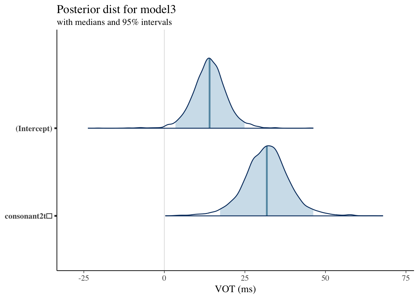
| (Intercept) | 13.9642848 | 0.1255139 | 5.2862739 | 3.1361188 | 11.0509740 | 13.9311869 | 17.0777707 | 24.691811 | 1774 | 0.9995626 |
| consonant2t̻ | 32.0826482 | 0.1900716 | 6.8916103 | 18.0067462 | 27.9681689 | 32.0435970 | 36.0816424 | 46.336768 | 1315 | 1.0033702 |
| b[(Intercept) speaker_id:F01] | -1.5302904 | 0.1213132 | 5.1595532 | -12.2904876 | -4.5585220 | -1.5071204 | 1.5791178 | 8.610477 | 1809 | 0.9996977 |
| b[consonant2t̻ speaker_id:F01] | -4.7768015 | 0.1594894 | 6.3289503 | -17.7257696 | -8.7602367 | -4.7047401 | -0.8222776 | 7.737750 | 1575 | 1.0022687 |
| b[(Intercept) speaker_id:F02] | -7.6194908 | 0.1193882 | 5.2272817 | -18.8686135 | -10.7747593 | -7.4814266 | -4.3411413 | 2.323210 | 1917 | 1.0000940 |
| b[consonant2t̻ speaker_id:F02] | 6.7769788 | 0.1547371 | 6.2980373 | -5.6811122 | 2.7948426 | 6.6968777 | 10.6883551 | 19.593682 | 1657 | 1.0020555 |
| b[(Intercept) speaker_id:M01] | 12.8219215 | 0.1269118 | 5.2120165 | 2.6440517 | 9.5812362 | 12.6441052 | 15.9817349 | 23.732545 | 1687 | 1.0001472 |
| b[consonant2t̻ speaker_id:M01] | -10.6726342 | 0.1551055 | 6.4239402 | -23.8206246 | -14.4838725 | -10.4911580 | -6.6159101 | 1.476965 | 1715 | 1.0021635 |
| b[(Intercept) speaker_id:M02] | -3.7475418 | 0.1178971 | 5.2498634 | -13.9676660 | -6.8412054 | -3.7694361 | -0.5812705 | 6.885174 | 1983 | 1.0005591 |
| b[consonant2t̻ speaker_id:M02] | -7.4626967 | 0.1438520 | 6.4531613 | -20.3668920 | -11.4871342 | -7.4374432 | -3.2859368 | 5.159041 | 2012 | 1.0026973 |
| b[(Intercept) speaker_id:M03] | 0.8052862 | 0.1194252 | 5.1499723 | -9.7182341 | -2.3057735 | 0.8143507 | 3.9433914 | 11.058106 | 1860 | 0.9998734 |
| b[consonant2t̻ speaker_id:M03] | 15.1600690 | 0.1717555 | 6.4186071 | 2.5838749 | 11.0604312 | 14.8079068 | 19.1281916 | 28.194856 | 1397 | 1.0017766 |
| b[(Intercept) word:ahdan] | -0.4639709 | 0.0384139 | 2.2340726 | -5.4803073 | -1.2297703 | -0.1988099 | 0.2850377 | 4.002418 | 3382 | 0.9997312 |
| b[consonant2t̻ word:ahdan] | 0.1216502 | 0.0598031 | 3.7822814 | -7.2350099 | -0.8235421 | 0.0063251 | 0.9773072 | 7.849380 | 4000 | 0.9993267 |
| b[(Intercept) word:ata] | -0.4843028 | 0.0456596 | 2.7196091 | -6.4657134 | -1.2464827 | -0.1866374 | 0.3818759 | 4.504693 | 3548 | 0.9992919 |
| b[consonant2t̻ word:ata] | -0.4672058 | 0.0546052 | 2.9632833 | -6.5674941 | -1.3714779 | -0.2005452 | 0.3459040 | 5.538544 | 2945 | 1.0001976 |
| b[(Intercept) word:idi] | 0.6035102 | 0.0401485 | 2.2781105 | -3.3654478 | -0.2866984 | 0.2329395 | 1.3053576 | 6.019724 | 3220 | 0.9991333 |
| b[consonant2t̻ word:idi] | -0.0003454 | 0.0738116 | 4.0638324 | -8.3097916 | -0.8763403 | 0.0043577 | 0.8040879 | 7.669826 | 3031 | 1.0004483 |
| b[(Intercept) word:itik] | 0.4689619 | 0.0459315 | 2.6030958 | -4.5123515 | -0.3572086 | 0.1811649 | 1.2375526 | 6.059717 | 3212 | 1.0012347 |
| b[consonant2t̻ word:itik] | 0.5790129 | 0.0597638 | 3.0314378 | -4.7012075 | -0.3587379 | 0.1818185 | 1.3865031 | 7.569620 | 2573 | 0.9991393 |
| sigma | 6.2668376 | 0.0107517 | 0.6799999 | 5.0720898 | 5.7877607 | 6.2122055 | 6.6877624 | 7.694882 | 4000 | 1.0000970 |
| Sigma[speaker_id:(Intercept),(Intercept)] | 109.4096891 | 2.1925481 | 97.1614838 | 22.3947189 | 51.0143263 | 81.5969220 | 132.6112301 | 358.757366 | 1964 | 1.0003071 |
| Sigma[speaker_id:consonant2t̻,(Intercept)] | -22.7260599 | 1.0912958 | 57.8124972 | -146.4107324 | -44.2173930 | -17.2813898 | 2.9971406 | 80.936666 | 2806 | 1.0020638 |
| Sigma[speaker_id:consonant2t̻,consonant2t̻] | 160.0292421 | 2.6974995 | 131.2439131 | 35.6382993 | 82.3131742 | 124.1417299 | 194.7151863 | 490.847653 | 2367 | 1.0006840 |
| Sigma[word:(Intercept),(Intercept)] | 9.9382626 | 0.5093796 | 28.1101736 | 0.0034933 | 0.3980251 | 2.0886674 | 7.9939197 | 76.805961 | 3045 | 0.9993027 |
| Sigma[word:consonant2t̻,(Intercept)] | -0.7197121 | 0.1922373 | 12.1581554 | -16.6219774 | -0.8116888 | -0.0036399 | 0.4309056 | 11.617087 | 4000 | 0.9995805 |
| Sigma[word:consonant2t̻,consonant2t̻] | 14.7685657 | 1.0254484 | 55.3351743 | 0.0028683 | 0.4427945 | 2.5722091 | 10.4894988 | 105.721342 | 2912 | 1.0001081 |
| mean_PPD | 30.8019709 | 0.0185724 | 1.1746229 | 28.4877981 | 30.0332389 | 30.7937003 | 31.5746953 | 33.088275 | 4000 | 0.9999336 |
| log-posterior | -240.5881277 | 0.1536367 | 4.9786412 | -251.3596254 | -243.7667338 | -240.2288973 | -237.1560916 | -231.899535 | 1050 | 1.0020654 |
Compared to frequentist model
model_freq <- lmer(vot*1000 ~ consonant2 + (1+consonant2|speaker_id) + (1+consonant2|word),data=data_vot)
sjPlot::sjt.lmer(model_freq)| vot * 1000 | ||||
| B | CI | p | ||
| Fixed Parts | ||||
| (Intercept) | 14.21 | 6.49 – 21.94 | .020 | |
| consonant2 (t̻) | 31.84 | 20.59 – 43.09 | .004 | |
| Random Parts | ||||
| σ2 | 36.684 | |||
| τ00, speaker_id | 70.586 | |||
| τ00, word | 0.143 | |||
| ρ01 | -0.499 | |||
| Nspeaker_id | 5 | |||
| Nword | 4 | |||
| ICCspeaker_id | 0.657 | |||
| ICCword | 0.001 | |||
| Observations | 58 | |||
| R2 / Ω02 | .916 / .916 | |||
| vot * 1000 | ||||
| B | CI | p | ||
| Fixed Parts | ||||
| (Intercept) | 14.21 | 6.49 – 21.94 | .020 | |
| consonant2 (t̻) | 31.84 | 20.59 – 43.09 | .004 | |
| Random Parts | ||||
| σ2 | 36.684 | |||
| τ00, speaker_id | 70.586 | |||
| τ00, word | 0.143 | |||
| ρ01 | -0.467 | |||
| Nspeaker_id | 5 | |||
| Nword | 4 | |||
| ICCspeaker_id | 0.657 | |||
| ICCword | 0.001 | |||
| Observations | 58 | |||
| R2 / Ω02 | .916 / .916 | |||
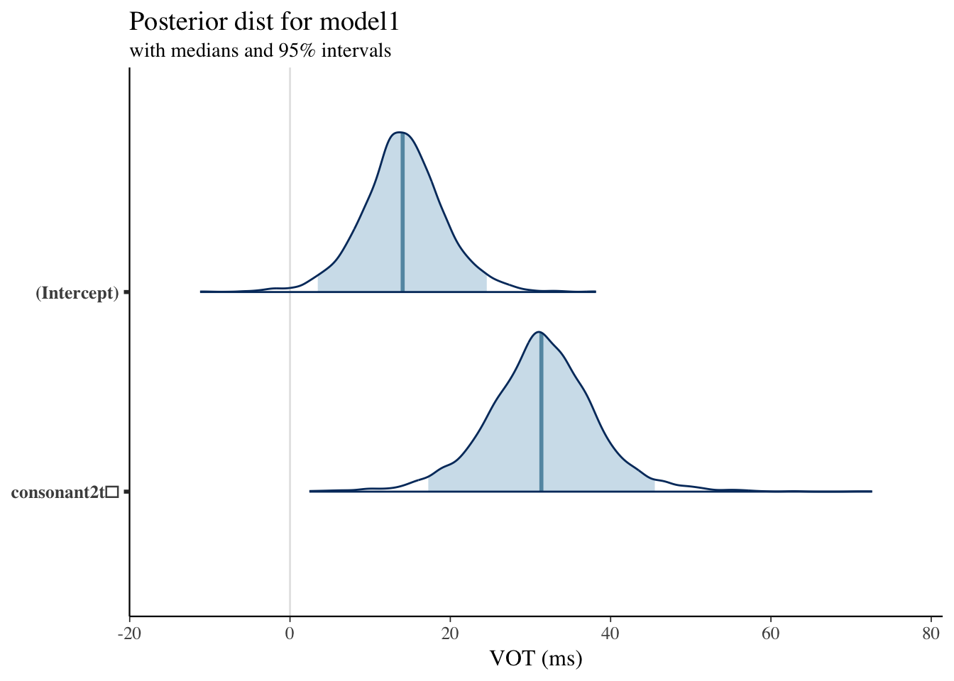
Plotting Posterior Distribution: Model1
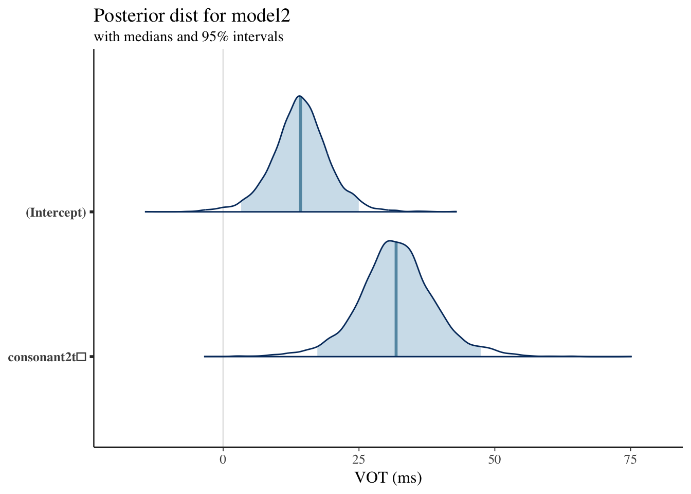
Plotting Posterior Distribution: Model2
Plotting Posterior Distribution: Model3
Diagnostics and Comparing Models
Model Diagnostics
- In summary output want Rhat to be 1.0 or very close to 1 (like 0.98) [measure of how well the chains mix]
- Use
launch_shinystan(model1)to explore Stan’s built in diagnostic tools (launches page in your web browser)
Example of Shinystan

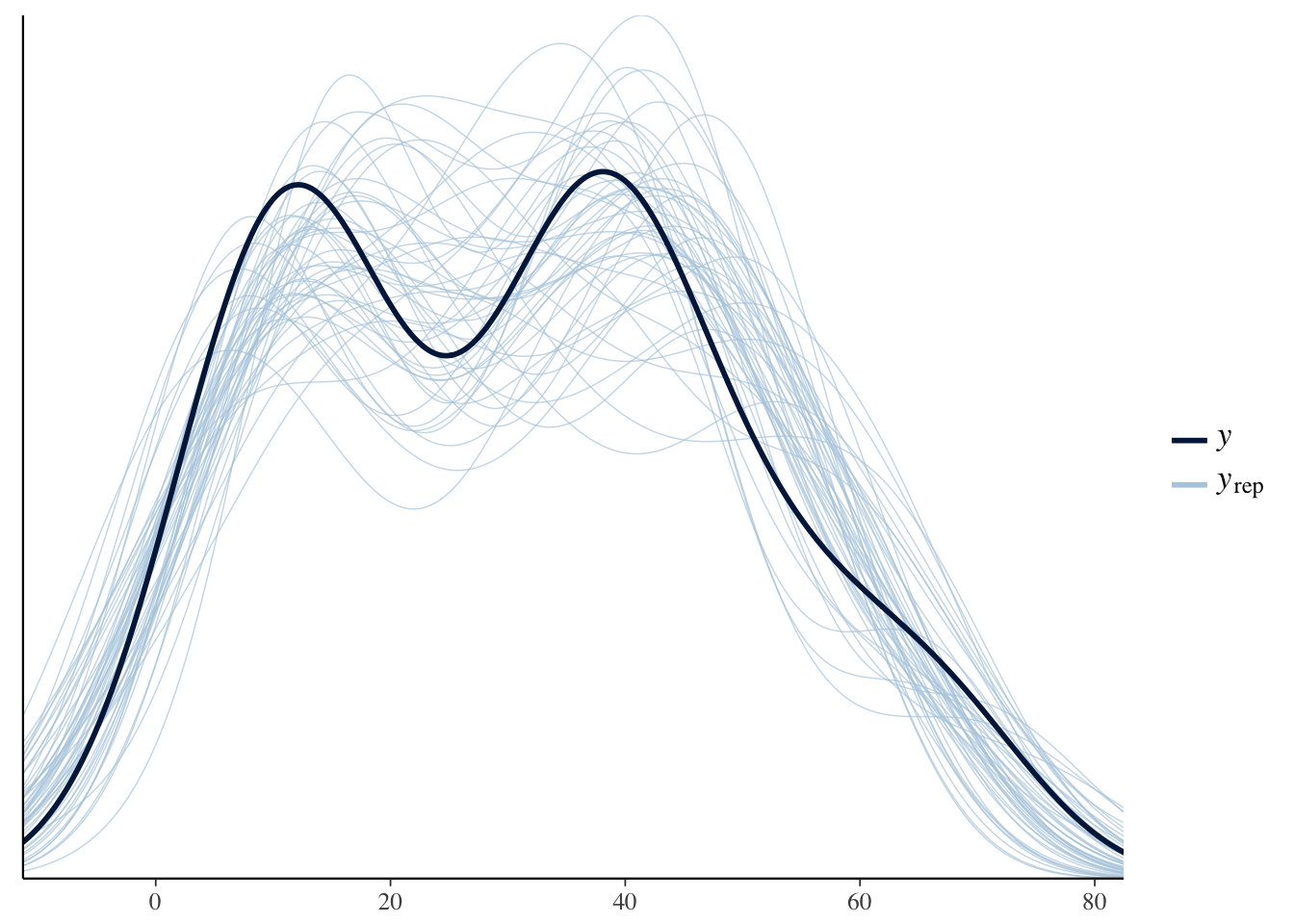
How well did the model sample
Model Comparisons
- Like frequentist models, we can compare two different models to see how different they are (like comparing random effects)
- Instead of
anova()we useloo()(leave one out) andcompare_models() - Can take a little bit to run
loo()is actually more like comparingAICvalues- If
elpd_diffis small, then little difference between models loois an approximation ofk_fold(model,K=10)but is much faster
Loo
- The LOO Information Criterion (LOOIC) has the same purpose as the Akaike Information Criterion (AIC) that is used by frequentists.
- Both are intended to estimate the expected log predictive density (ELPD) for a new dataset.
- However, the AIC ignores priors and assumes that the posterior distribution is multivariate normal, whereas the functions from the loo package do not make this distributional assumption and integrate over uncertainty in the parameters.
- This only assumes that any one observation can be omitted without having a major effect on the posterior distribution
ELPD
- The difference in ELPD will be negative if the expected out-of-sample predictive accuracy of the first model is higher.
- If the difference is be positive then the second model is preferred.
Example loo
model1a <-stan_lmer(vot*1000 ~ consonant2 + (1+consonant2|speaker_id),
data=data_vot,
prior_intercept = normal(0, 5),
prior = normal(0, 5),
prior_covariance = decov(regularization = 2),
chains = 4,
iter = 2000, adapt_delta=0.999,warmup=1000)

loo1 <- loo(model1)
loo1a <- loo(model1a)
Compare models
compare_models(loo1,loo1a)## elpd_diff se
## 0.4 1.1Summary
Pros and cons of Bayesian analyses
- Pros
- Easier to intrpret
- No p-values
- Uses past knowledge (more scientific)
- Can use more complex models
- Can do multiple comparisons
- Have distributions of results
- Can make more nuanced claims
- Cons
- Slower
- New for linguistics so have to explain more