What to do with categorical data?
- Categorical data can be challenging to analyze quantitatively
- In language research we often have data that are purely categorical
- In today’s presentation we will deal with a specific type of categorical data found in questionnaires
Questionnaire Data
- Questionnaires are frequently used in a variety of language research scenarios
- They often ask people to rate something (likert scales) or select the most appropriate response
- There are often multiple questions that have the same answer scale (same choices)
- Example: select the language that is most appropriate to use in a given domain
- Example: rate level of agreement with several statements
Research Question
- Often we are interested in how the questions relate to each other in terms of their answers as well as how the answers relate to each other based on the questions they were most used with
Correspondence Analysis
- CA is statistical technique that shows how the questions and answers of multiple questions relate to each other
- Requires the data to have the same scale (all questions must have some possible answers)
- CA is a descriptive tool and doesn’t give p-values per se
How does CA work?
- CA takes a series of categorical variables and converts them to a contingency table (a count of the number of responses at each level for each variable)
- It then uses the chi-squared distribution to convert the data into a series of factors (you can specify the number of factors)
- These factors are designed to be minimally correlated with each other
- The first factor represents the most variation in the data and the following ones less so
- It takes a large number of variables and maps them on to a smaller number of variables
- Very similar to Principle Component Analysis (PCA)
Example Data
- For the sample CA, we will be using data from a language attitudes questionnaire used on Pohnpei (PNI) in the Federated States of Micronesia
- The selected data come from 25 questions where the respondents were asked to select the 1 language (out of 8 possible answers) that is the most important for that specific domain
- The answers for all 25 questions were the same 8 language choices
domains <- read.csv("domains.csv")
Explore the data
| English |
English |
English |
English |
English |
English |
English |
English |
English |
English |
English |
English |
English |
English |
Other |
English |
English |
English |
English |
English |
English |
English |
English |
English |
Other |
| Pohnpeian |
Pohnpeian |
Pohnpeian |
Pohnpeian |
Pohnpeian |
Pingelapese |
Pohnpeian |
Pohnpeian |
Pohnpeian |
Pohnpeian |
Pohnpeian |
Pohnpeian |
Pohnpeian |
Pohnpeian |
Pohnpeian |
Pohnpeian |
Pohnpeian |
Pohnpeian |
Pohnpeian |
Pohnpeian |
Pohnpeian |
Pohnpeian |
Pohnpeian |
Pohnpeian |
Pohnpeian |
| Pohnpeian |
English |
English |
Pohnpeian |
English |
English |
English |
English |
English |
Pohnpeian |
Pohnpeian |
Pohnpeian |
Pohnpeian |
Pohnpeian |
Pohnpeian |
English |
Pohnpeian |
Pohnpeian |
English |
English |
Pohnpeian |
Pohnpeian |
Pohnpeian |
Pohnpeian |
English |
| Pohnpeian |
English |
English |
English |
English |
English |
English |
English |
English |
Pohnpeian |
English |
English |
Pohnpeian |
Pohnpeian |
Pohnpeian |
Pohnpeian |
Pohnpeian |
Pohnpeian |
English |
English |
English |
Pohnpeian |
Pohnpeian |
Pohnpeian |
Pohnpeian |
| English |
English |
English |
English |
English |
English |
English |
English |
English |
Pohnpeian |
English |
Pohnpeian |
Pohnpeian |
Pohnpeian |
Pohnpeian |
English |
Pohnpeian |
Pohnpeian |
Pohnpeian |
English |
English |
Pohnpeian |
Pohnpeian |
Pohnpeian |
English |
| Pohnpeian |
English |
English |
Pohnpeian |
English |
English |
English |
English |
English |
Pohnpeian |
English |
Pohnpeian |
Pohnpeian |
Pohnpeian |
Pohnpeian |
English |
Pohnpeian |
Pohnpeian |
Pohnpeian |
English |
English |
Pohnpeian |
Pohnpeian |
Pohnpeian |
English |
Step 1: Create contingency table
library(tidyverse)
domains.gathered <- domains %>% gather(key=domain,value=language)
domains.gathered$domain <- as.factor(domains.gathered$domain)
domains.gathered$language <- as.factor(domains.gathered$language)
dt <- with(domains.gathered,table(domain,language))
| accepted_pni |
0 |
93 |
2 |
0 |
0 |
4 |
1 |
201 |
| being_successful |
0 |
179 |
1 |
0 |
1 |
3 |
0 |
117 |
| church |
2 |
43 |
8 |
6 |
6 |
5 |
6 |
225 |
| facebook |
1 |
138 |
4 |
1 |
0 |
4 |
5 |
148 |
| friends_school |
1 |
100 |
1 |
0 |
0 |
5 |
1 |
193 |
| funerals |
2 |
20 |
0 |
2 |
1 |
3 |
2 |
271 |
| getting_money |
0 |
176 |
2 |
1 |
1 |
4 |
1 |
116 |
| good_education |
0 |
194 |
0 |
2 |
1 |
5 |
0 |
99 |
| good_job |
1 |
178 |
2 |
0 |
1 |
7 |
1 |
111 |
| happy_relationships |
3 |
91 |
4 |
6 |
7 |
9 |
3 |
178 |
| kamadipw |
2 |
42 |
1 |
2 |
1 |
3 |
2 |
248 |
| making_friends |
0 |
101 |
1 |
0 |
4 |
3 |
2 |
190 |
| radio |
1 |
124 |
6 |
0 |
1 |
2 |
0 |
167 |
| reading |
0 |
175 |
1 |
0 |
2 |
0 |
2 |
121 |
| sakau |
0 |
23 |
1 |
1 |
1 |
2 |
3 |
270 |
| store |
1 |
63 |
2 |
1 |
2 |
4 |
3 |
225 |
| talking_chief |
0 |
16 |
1 |
0 |
2 |
2 |
3 |
277 |
| talking_gov |
0 |
134 |
0 |
0 |
1 |
4 |
0 |
162 |
| talking_kolonia |
0 |
48 |
1 |
0 |
0 |
4 |
3 |
245 |
| talking_neighbors |
4 |
70 |
3 |
3 |
5 |
4 |
5 |
207 |
| talking_teachers |
0 |
183 |
2 |
0 |
2 |
3 |
0 |
111 |
| talking_villages |
0 |
22 |
1 |
1 |
1 |
2 |
1 |
273 |
| tv |
1 |
206 |
3 |
1 |
0 |
8 |
0 |
82 |
| us_relatives |
5 |
107 |
1 |
4 |
4 |
7 |
6 |
167 |
| writing |
0 |
179 |
2 |
0 |
1 |
6 |
2 |
111 |
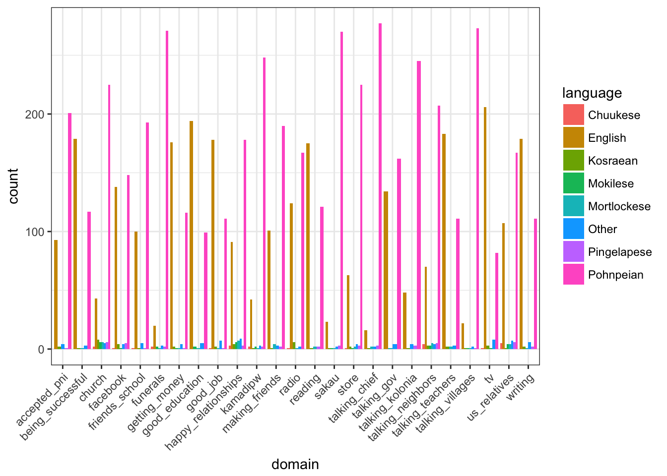
Plot raw data
Step 2: Run the CA
library(FactoMineR)
library(factoextra)
domains.CA <- CA(dt, graph=F)
Step 3: Visualize the CA (symmetric)
fviz_ca_biplot(domains.CA,repel=T)
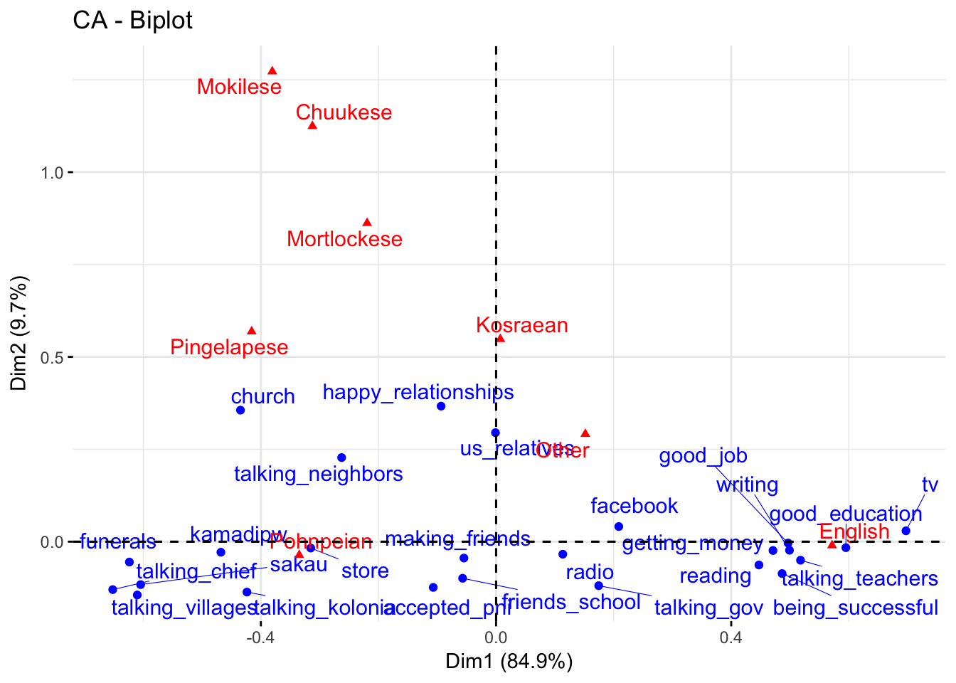
Symmetric vs asymmetric plots
- In the symmetric plot both columns are rows are plotted on same space
- The problem is that only the distance between the row points and other row points and the distance between the columns points and other column points are directly interpretable and NOT the distance between columns and rows
- To intrepret the distance between columns and row, we have to create an asymmetric plot where either the columns are mapped onto row space or rows mapped onto column space
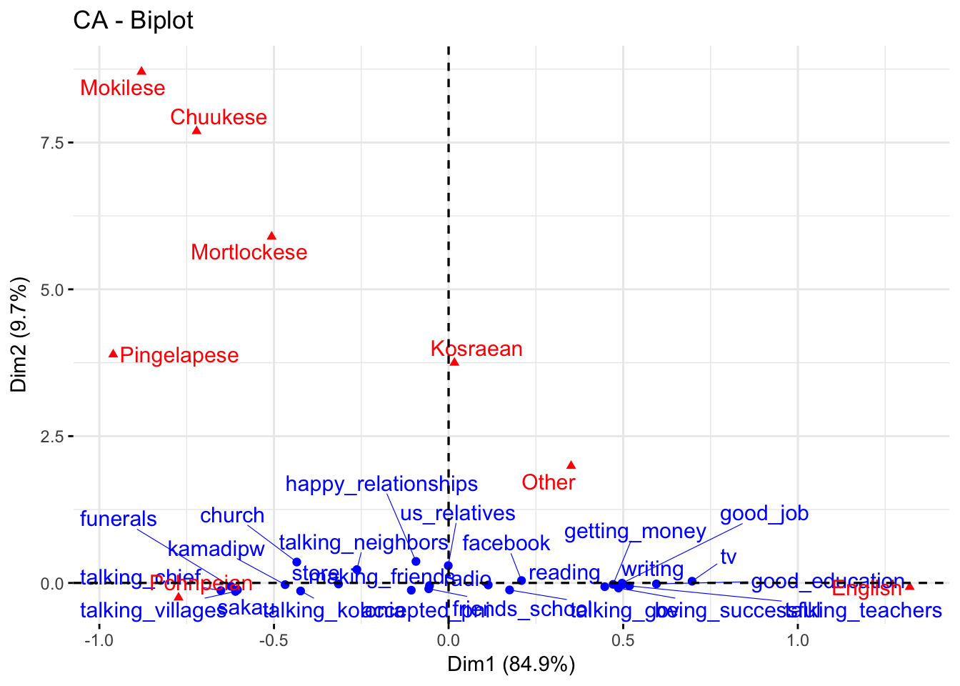
Asymmetric plot (row space)
fviz_ca_biplot(domains.CA,repel=T,map="rowprincipal")
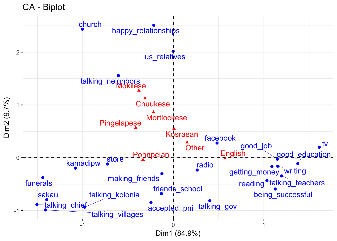
Asymmetric plot (column space)
fviz_ca_biplot(domains.CA,repel=T,map="colprincipal")
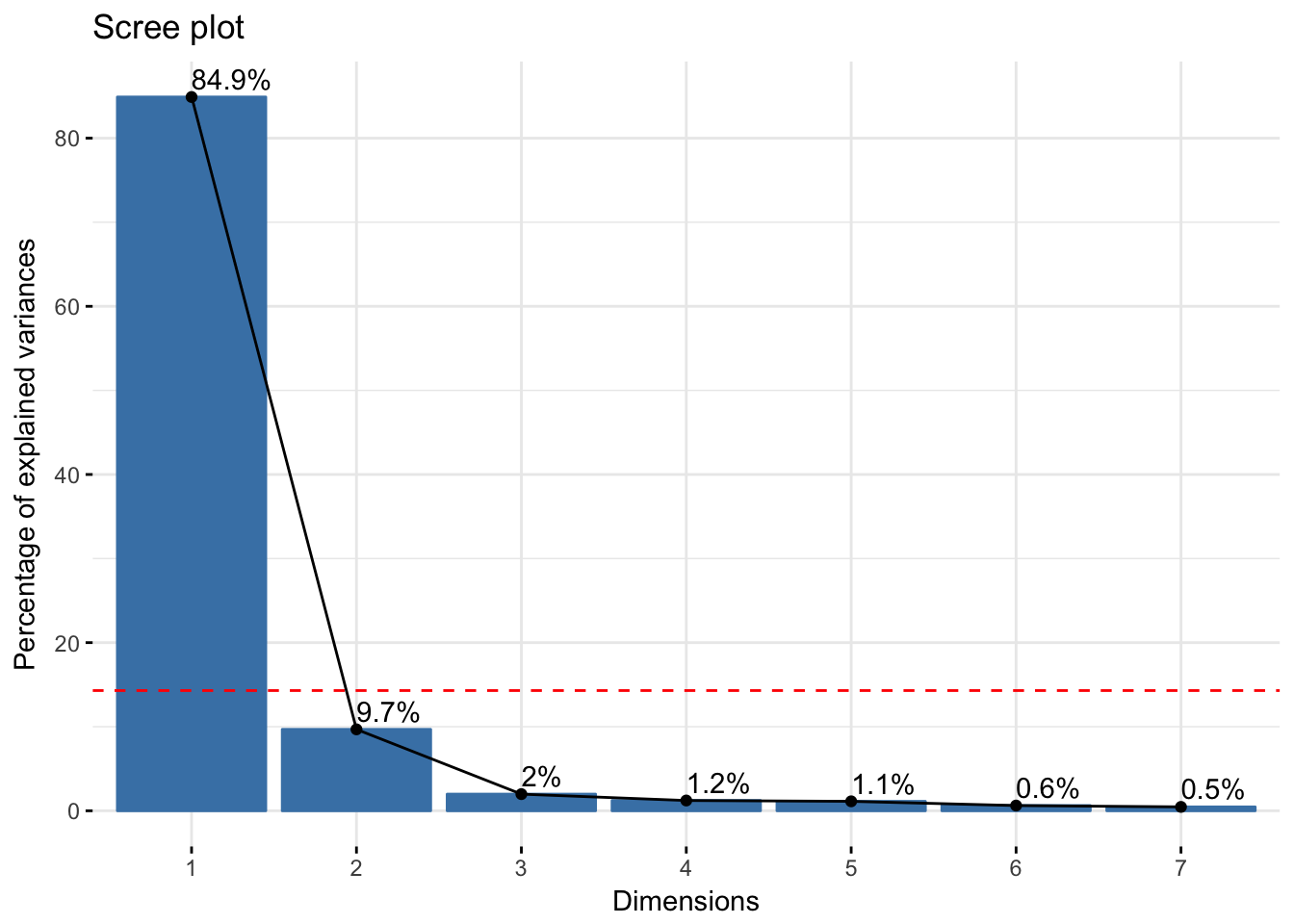
Step 4: How many axes do we keep?
- The CA created many possible axes, but only some are helpful
- Each axis has an eigenvalue that tell us how much information it explains (larger eigenvalue, more info)
- If the data were completely random, we’d expect each axis to have an eigenvalue of
1/(nrow(dt)-1) or \(1(25-1) = 1/24 = 4.2\%\) for rows and 1/(ncol(dt)-1) or \(1/(8-1) = 1/7 = 14.3\%\) for columns
- If eigenvalues are less than the largest of these two values, then should be kept, else can be ignored (though can keep it but will add little)
- For us, we look for eigenvalues 14.3% or greater
Exploring Eigenvalues
fviz_screeplot(domains.CA,addlabels=T) +
  geom_hline(yintercept=14.3,linetype=2,color="red")
Step 5: Interpreting axes
- The axes of the CA are not always immediately interpretable
- To better understand them, we look at which columns and which rows contributed the most to the creation of that axis
- We only need to explore axis 1, but will show axis 2 for sake of explanation
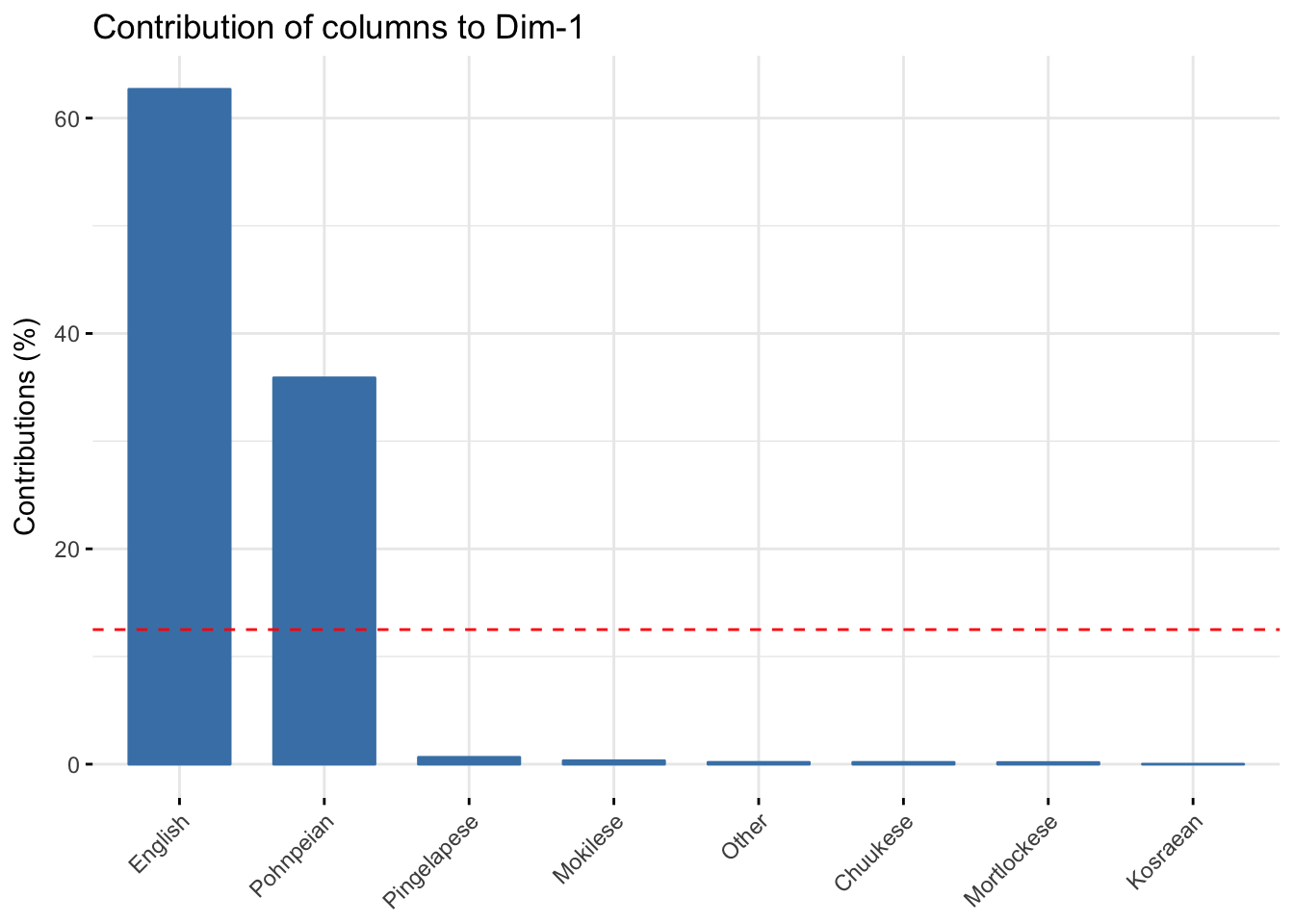
Columns contributing to axis 1
fviz_contrib(domains.CA, choice="col",axes=1)
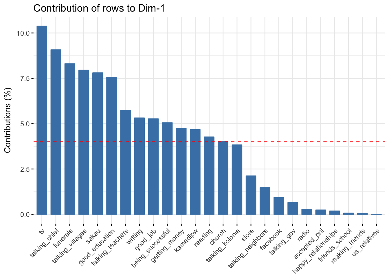
Rows contributing to axis 1
fviz_contrib(domains.CA, choice="row",axes=1)
Meaning of axis 1
- English and Pohnpeian contributed strongly to axis 1
- English and Pohnpeian are also on opposite sides
- Positive values of axis 1 correlate with more English and negative values with more Pohnpeian
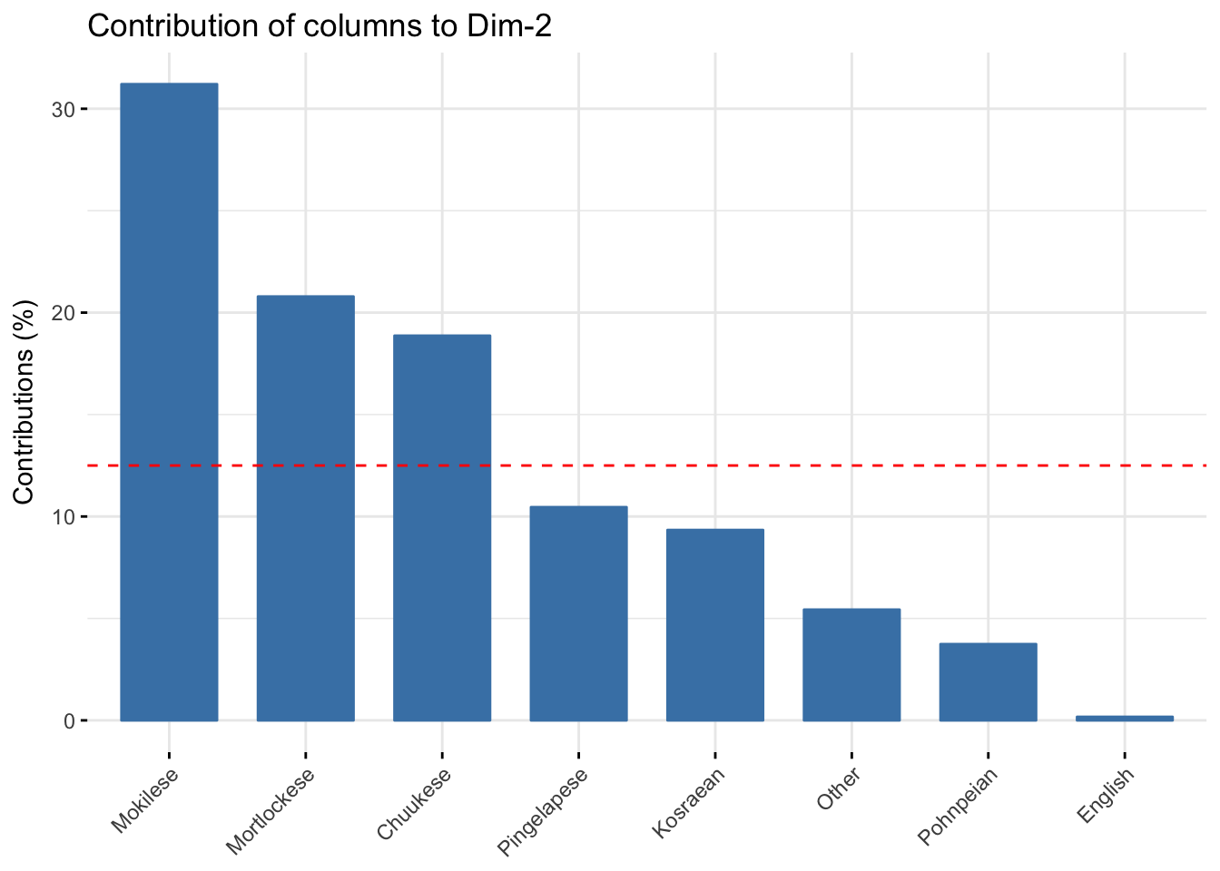
Columns contributing to axis 2
fviz_contrib(domains.CA, choice="col",axes=2)
Rows contributing to axis 2
fviz_contrib(domains.CA, choice="row",axes=2)
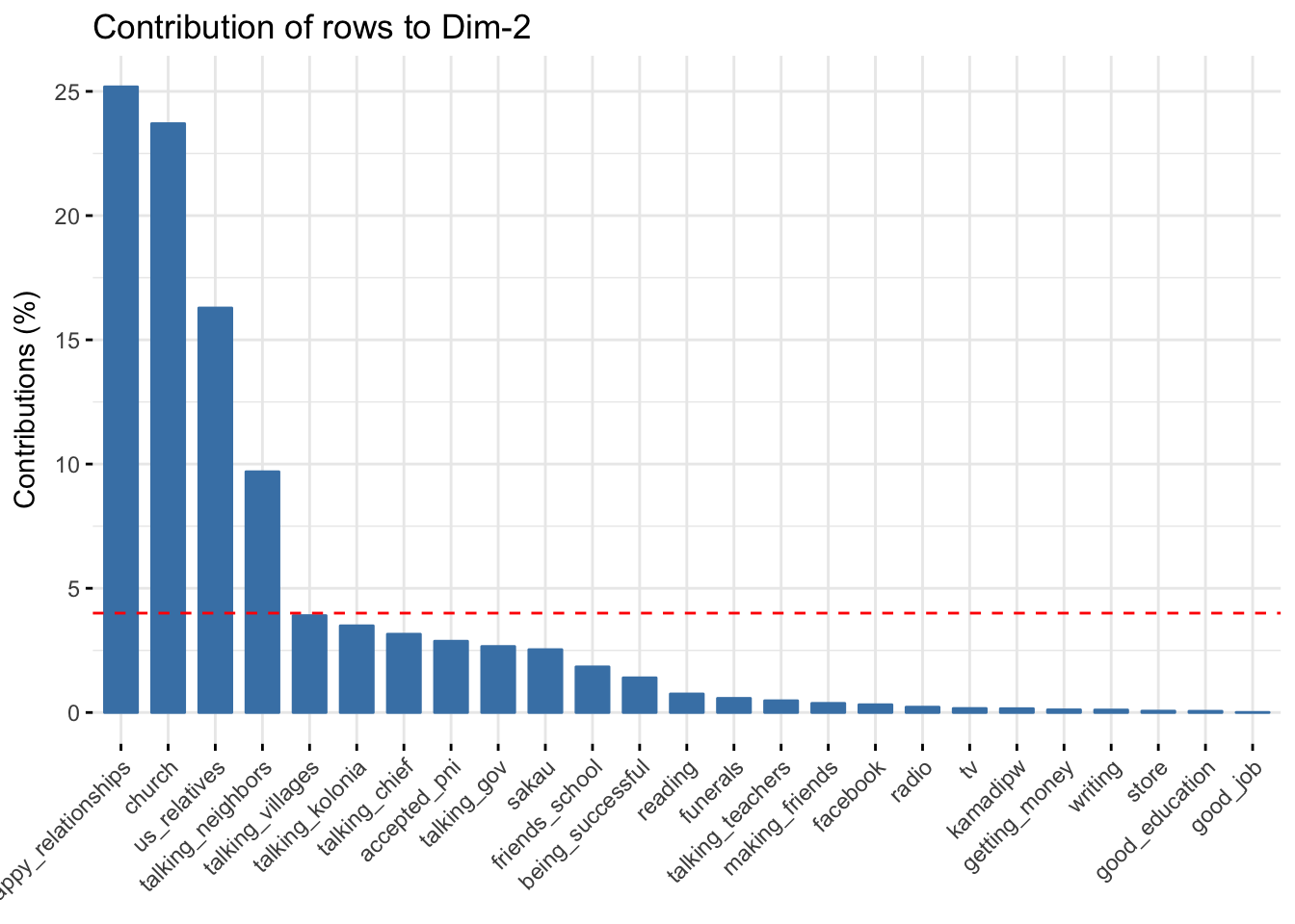
Meaning of axis 2
- Mokilese, Mortlockese, and Chuukese contributed strongly to axis 2
- They are all on thesame side of axis 2
- Positive values of axis 2 correlate with more values of Mokilese, Mortlockese, and Chuukese
Step 6: Evaluating quality of fit
- After determining the number of axes to retain and what they mean, we need to see how well each row and column item is represented by the retained number of dimensions
- The squared cosine (cos2) is a measure of the quality of representation
- cos2 values range from 0 to 1 and values close to 1 indicate a good representation and 0 a very bad representation
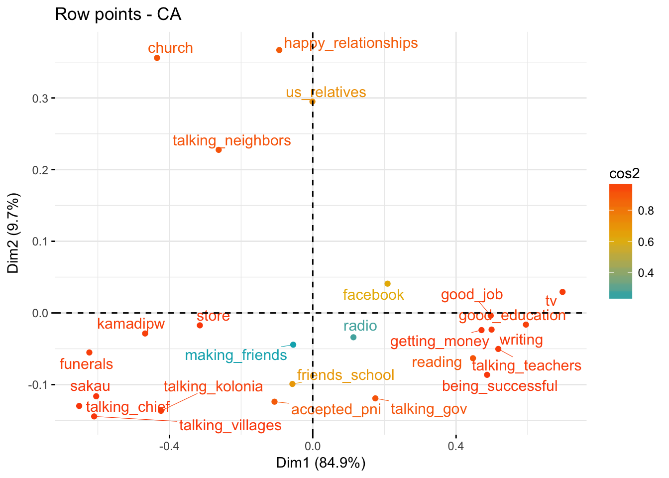
Quality of fit for rows
fviz_ca_row(domains.CA, col.row = "cos2",
             gradient.cols = c("#00AFBB", "#E7B800", "#FC4E07"),
             repel = TRUE)
Quality of fit for columns
fviz_ca_col(domains.CA, col.col = "cos2",
             gradient.cols = c("#00AFBB", "#E7B800", "#FC4E07"),
             repel = TRUE)
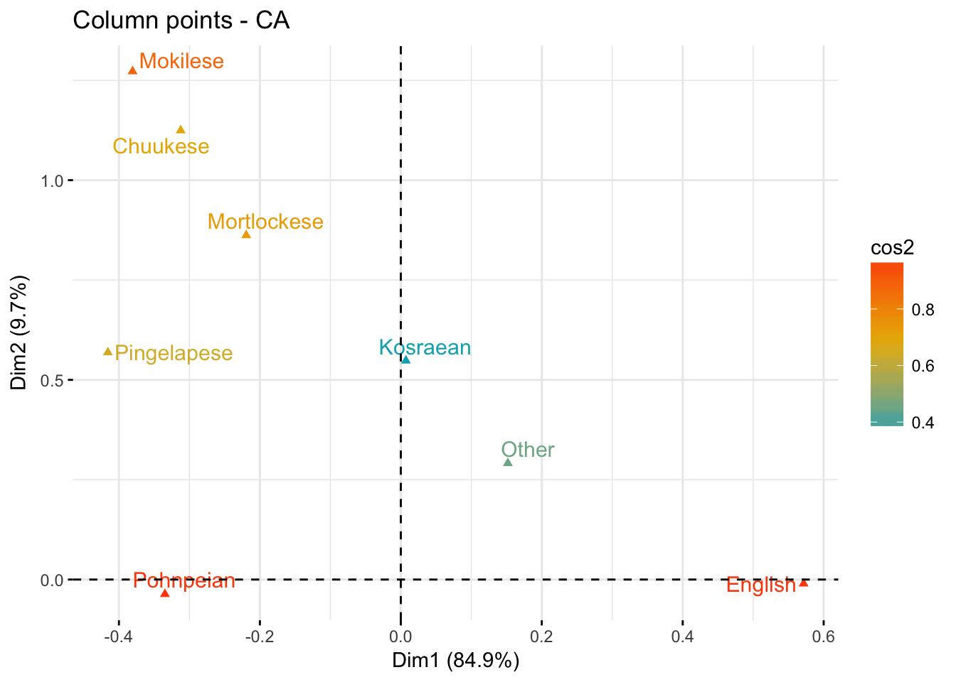
Quality of fit
- Rows making friends and radio have the lowest quality of fit for rows
- Columns Kosraean and other have the lowest quality of fit for columns
- That means that extra axes would better explain them
Step 7: Clustering the results
- This optional step allows you to cluster the rows together using hierachical clustering
- By specifying -1 clusters, the algorith automatically chooses the number of clusters for you based off the data
domains.CA.cluster <- HCPC(domains.CA,nb.clust=-1,graph=F)
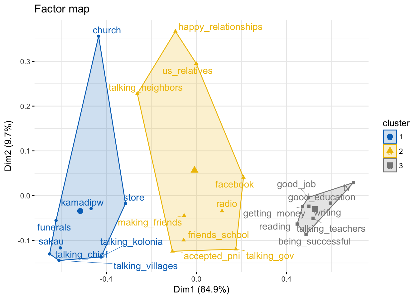
Visualizing clusters
fviz_cluster(domains.CA.cluster,
             repel = TRUE,
             show.clust.cent = TRUE,
             palette = "jco",
             ggtheme = theme_minimal(),
             main = "Factor map"
             )
Visualizing clusters
Another visualization
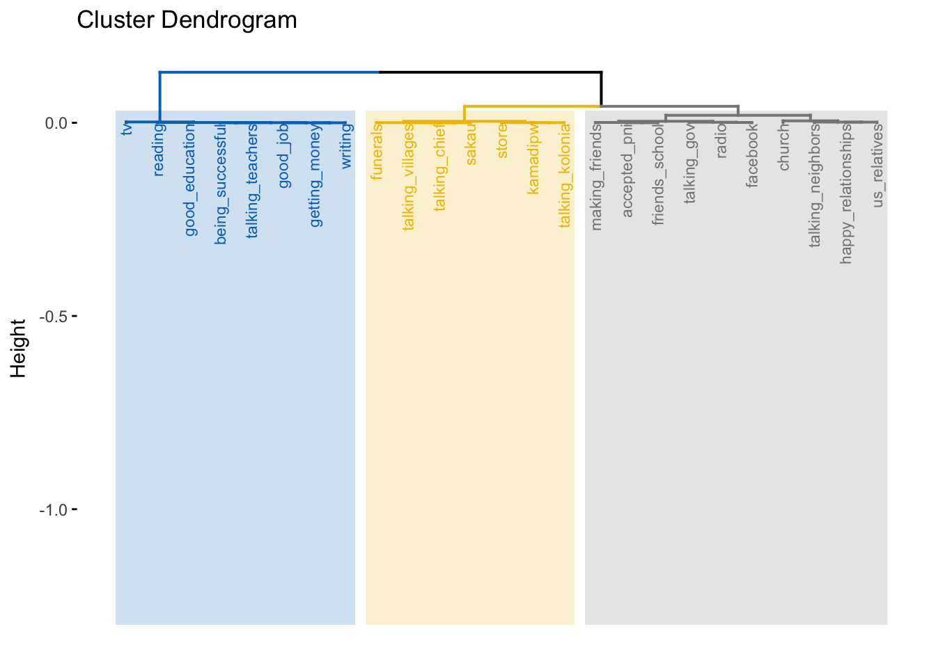
fviz_dend(domains.CA.cluster,
          cex = 0.7,
          palette = "jco",
          rect = TRUE, rect_fill = TRUE,
          rect_border = "jco",
          labels_track_height = 0.8
          )
Another visualization
Step 8: Interpretation of results
- Overall axis 1 indicates domains with more English selections (positive values) or more Pohnpeian selections (negative values)
- 5 of the 8 languages occur on the negative side of axis 1 so co-occur often with Pohnpeian domains
- No other languages are close to English on axis 1
- Cluster 1 includes domains that have high levels of Pohnpeian and other languages
- Cluster 2 include domains with mixed English and Pohnpeian (as well as other languages)
- Cluster 3 mostly English
Benefit of CA
- For this data, allows us to see (1) what languages pattern in similar ways, (2) what domains pattern in similar ways, and (3) how languages and domains interact
- Would be harder to see these patterns without CA
Automating CA
- The CA analysis can be automated somewhat (doesn’t always work)
- Just input the CA object and the function can create a sample analysis
- Outputs an html, Word doc, or pdf file
library(FactoInvestigate)
Investigate(domains.CA,document="html_document")
Now try it yourself
- Trying doing a CA analysis with
data(housetask)
- It is already a contigency table so can skip the first step